Statistical functions in R are used for statistical computations/analysis of a dataset.
Some statistical functions are already defined in R (these are built-in functions also known as
system-defined functions)
For all other functions not built-in, we have to define them. These are known as user-defined
functions.
As at today: 07/05/2023;
R programming language has these descriptive statistics represented by these built-in functions.
Let us review them.
| Descriptive Statistics | Type | Built-in R Function | Code |
|---|---|---|---|
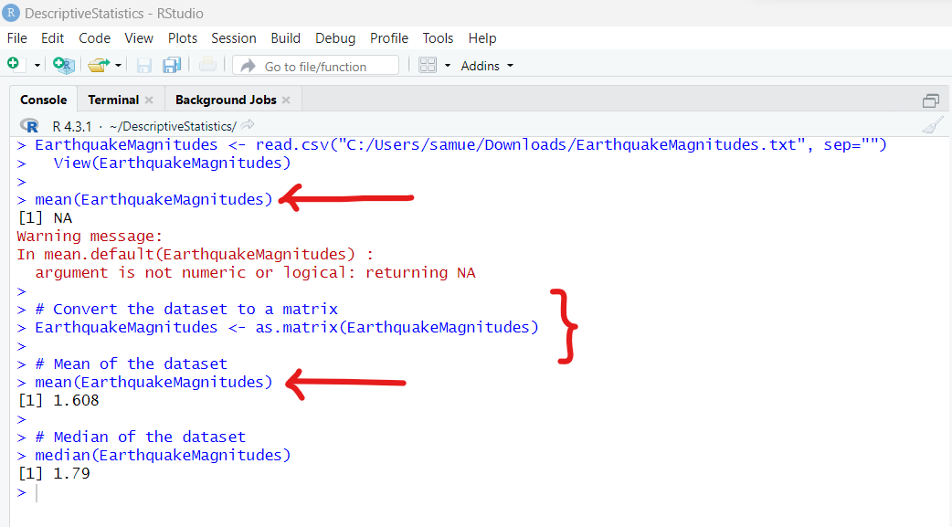
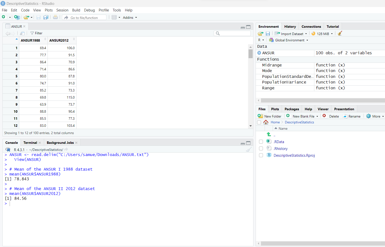
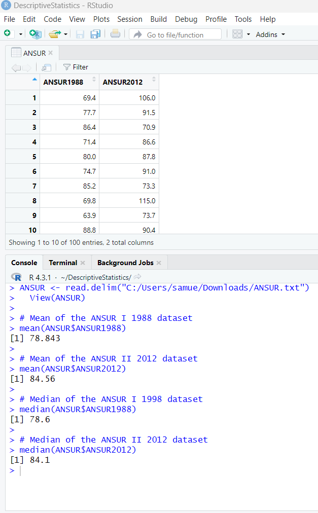
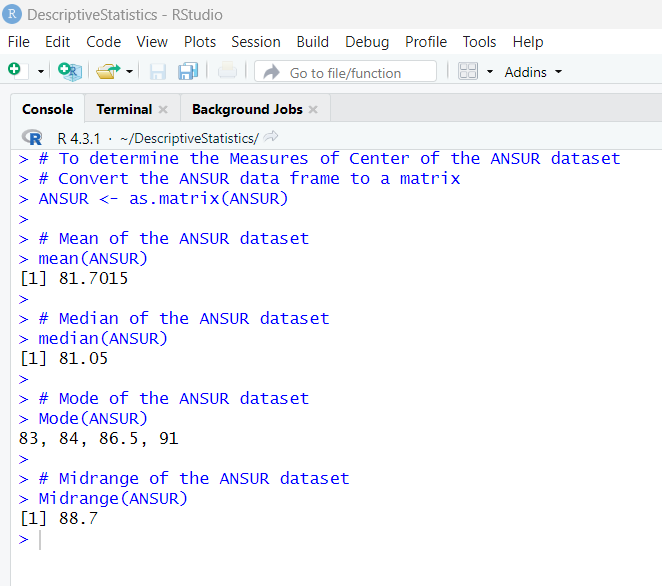
| Mean | Measure of Center | mean | mean(dataset) |
| Median | Measure of Center | median | median(dataset) |
| Sample Variance | Measure of Spread | var | var(dataset) |
| Sample Standard Deviation | Measure of Spread | sd | sd(dataset) |
| Five-Number Summary | Measure of Location | quantile | quantile(dataset) |
| Minimum | Measure of Location | min | min(dataset) |
| Maximum | Measure of Location | max | max(dataset) |
| Percentile (Example: 70th percentile) | Measure of Location | quantile | quantile(dataset, c(0.7)) |
| Percentiles (Example: 34th and 70th percentiles) | Measure of Location | quantile | quantile(dataset, c(0.34, 0.7)) |
This means that:
(1.) We cannot use the built-in function names as names for any user-defined variable or user-defined
function.
(2.) We have to define our own functions (user-defined functions) for any function that is not built-in.
In that sense, we shall:
(a.) create a project in RStudio
(b.) define all those functions in the project
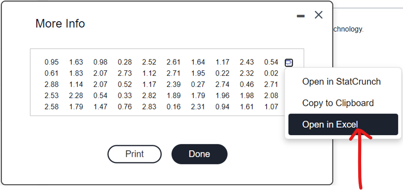
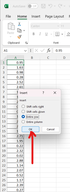
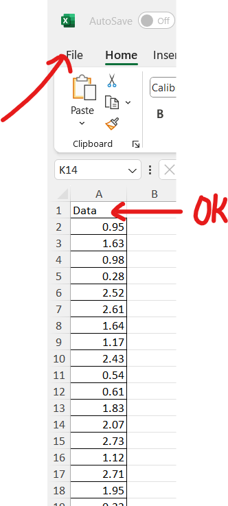
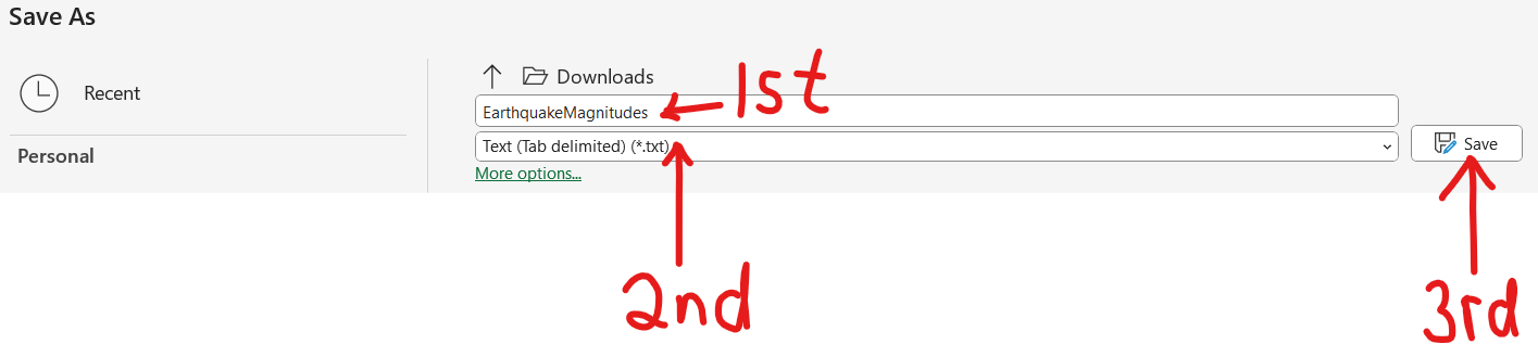
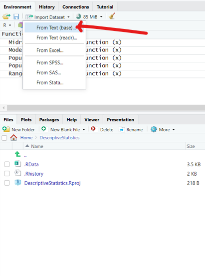
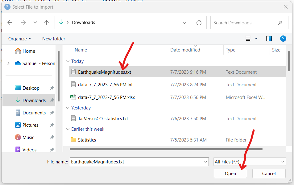
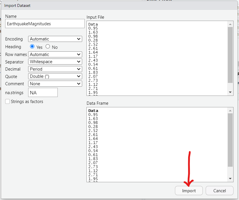
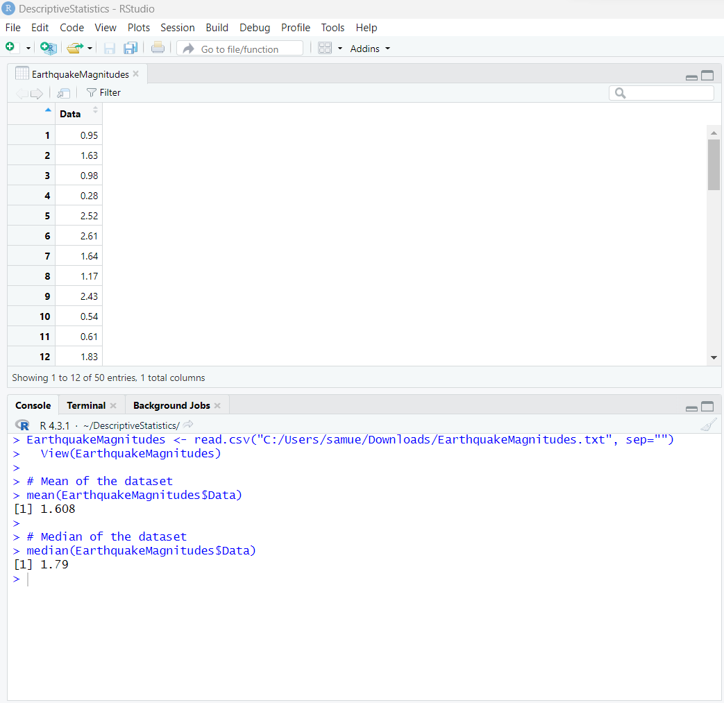
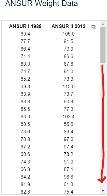
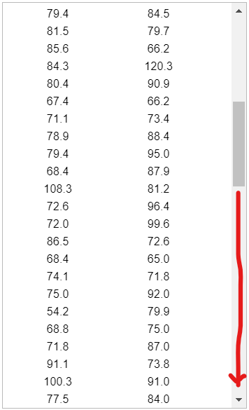
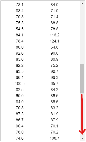
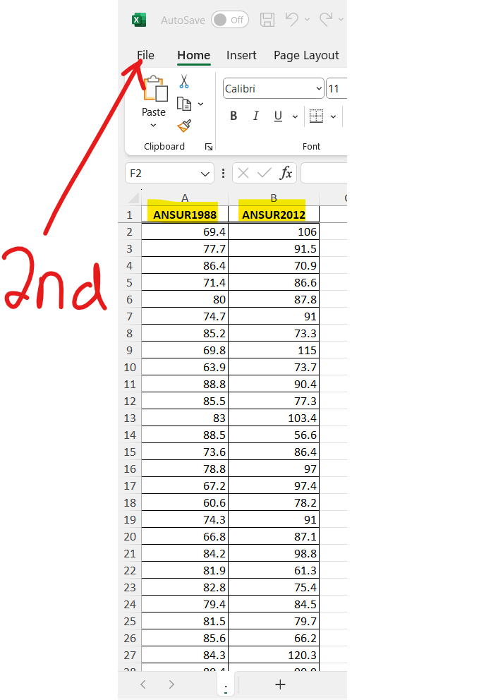
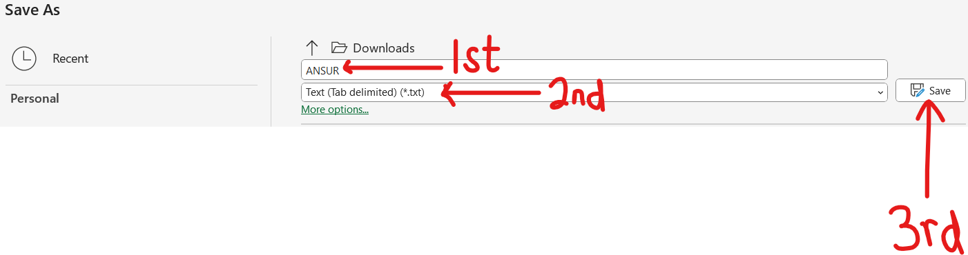
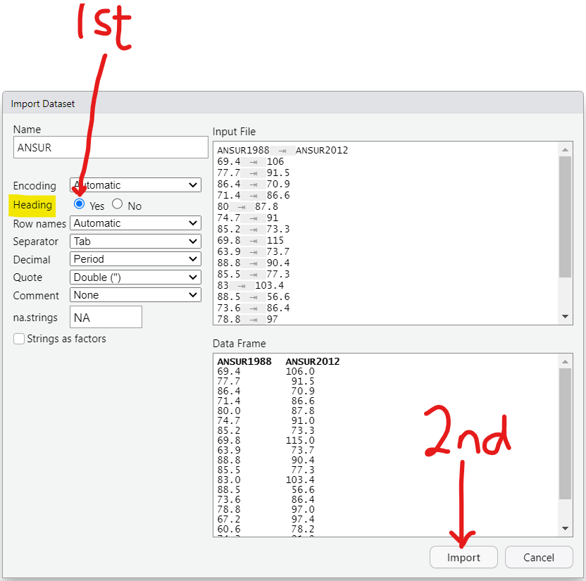
(c.) import any dataset we want into the project and use those functions in the dataset.
Create a Project in RStudio
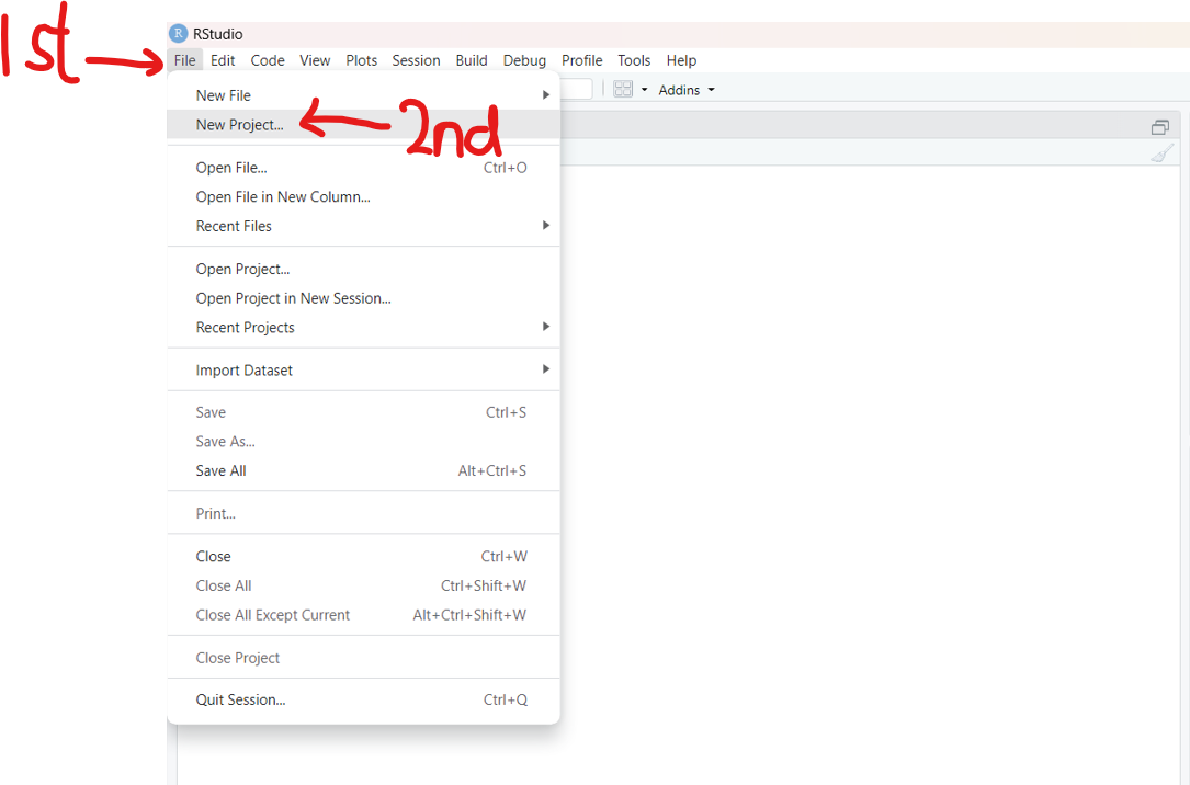
(1.) Step 1: Open RStudio
Click: File → New Project...
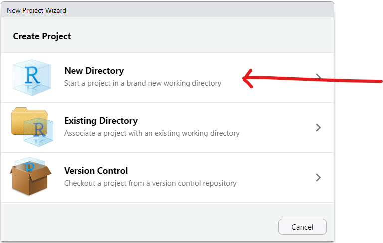
(2.) Step 2:
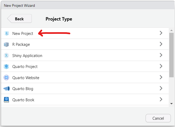
(3.) Step 3:
(4.) Step 4:
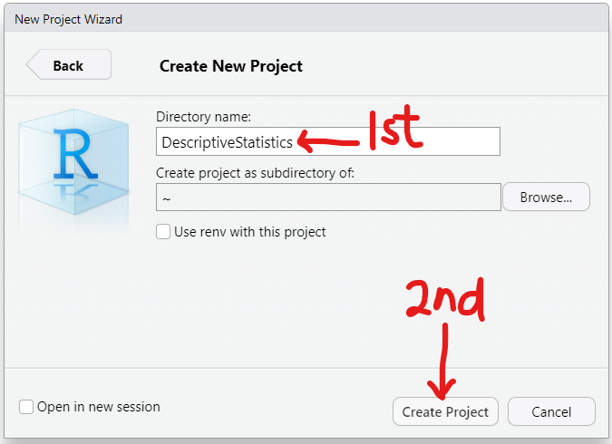
(5.) Step 5:
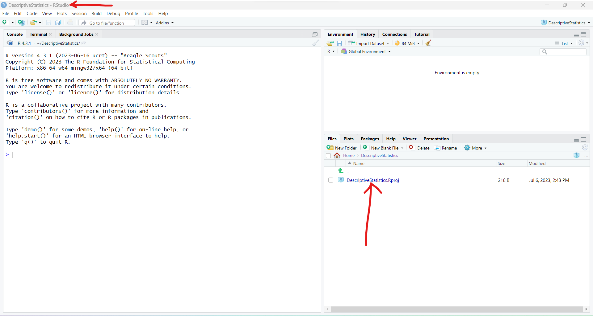
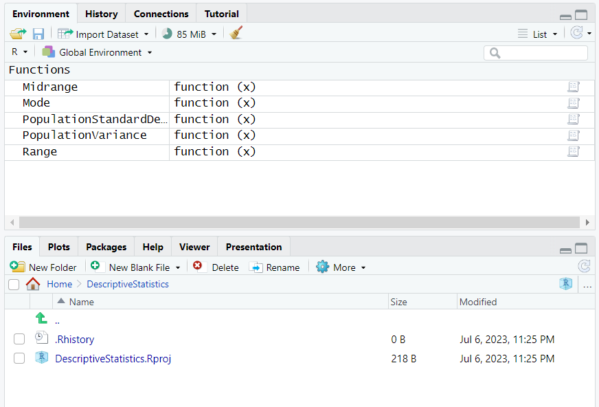
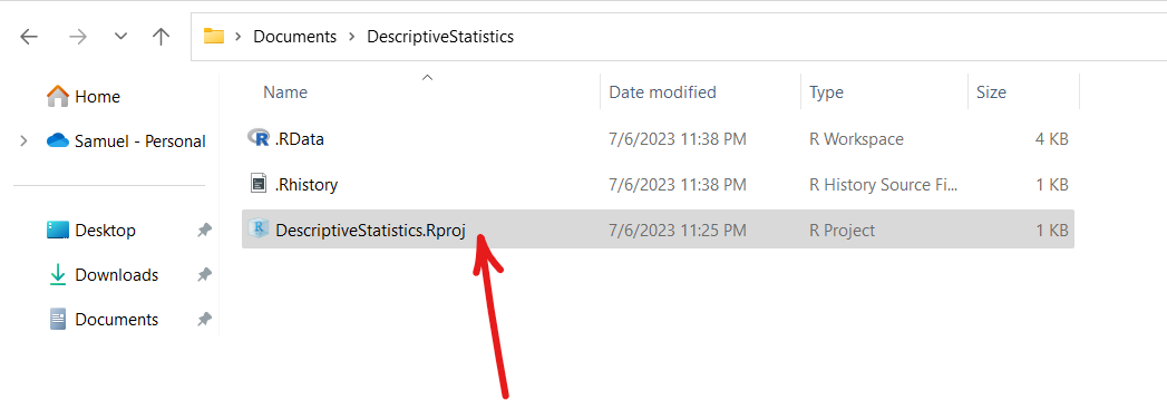
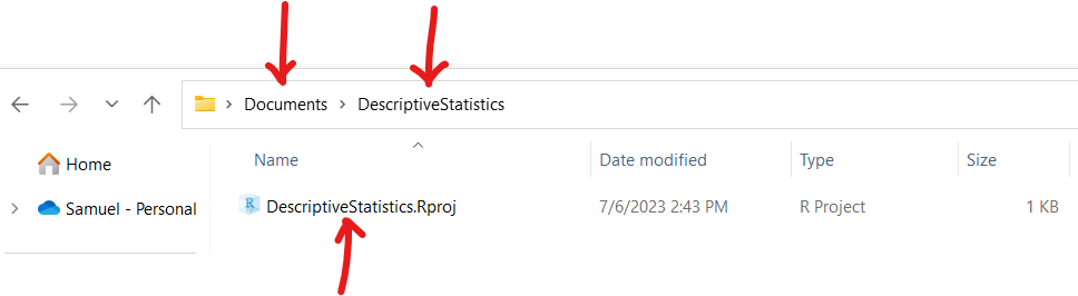
The project has been created.
By default, this project is located in the Documents folder of the Windows computer
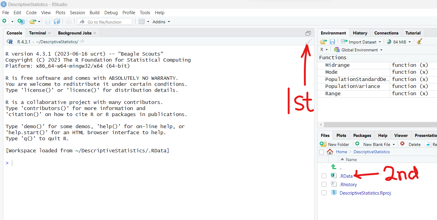
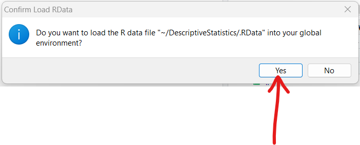
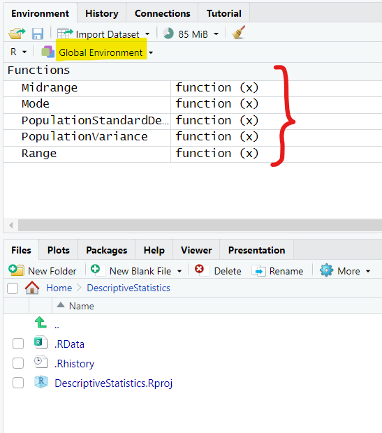
(6.) Step 6:
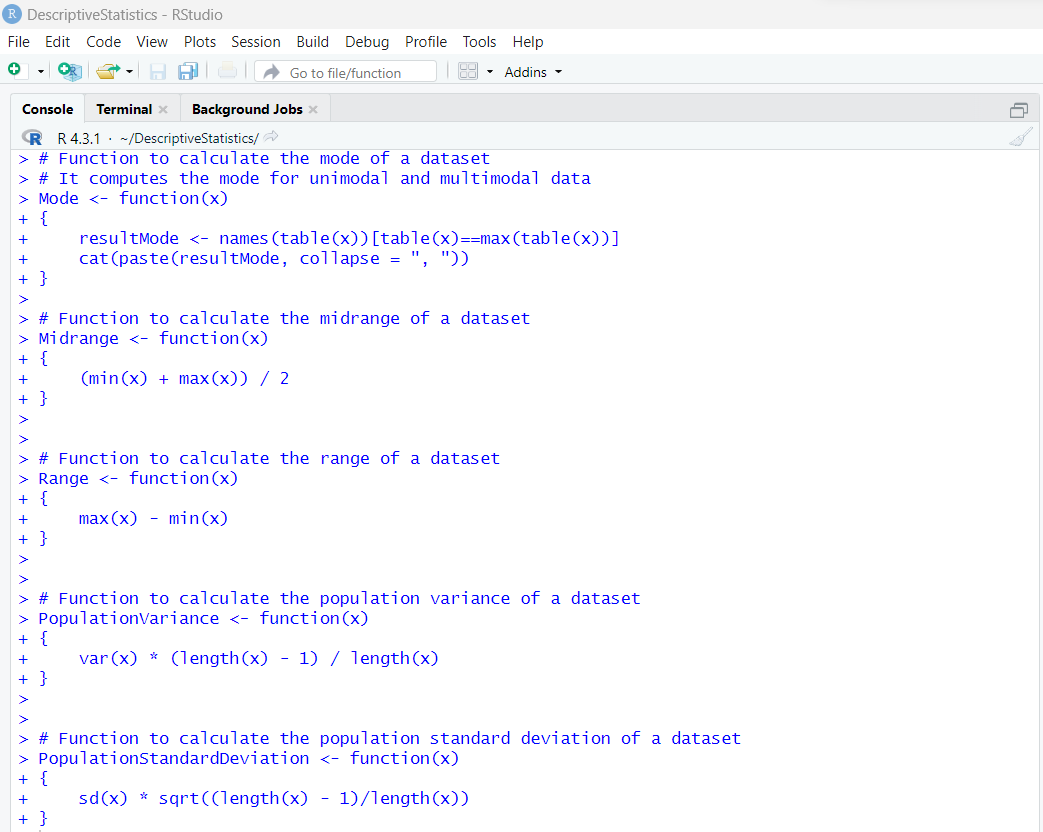
Let us go ahead and clear the default notes in the RStudio Console and let us write the
remaining statistical functions.